Equivalent source characteristics
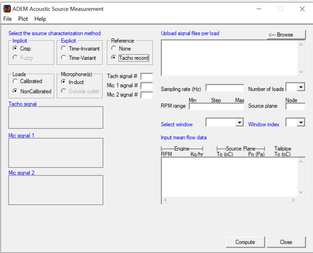
Microphone time-signals recorded in calibrated or non-calibrated multi-load tests can be imported and processed for the calculation of the pressure strength and impedance of one-port sources. The following methods can be implemented from the user interface shown in Figure 1:
Two-load method
Assumes time-invariant, load-independent source. Requires a reference signal from the source. Load over-determination can be used for statistical smoothing of measurement errors. Tests can be steady or non-steady.
Explicit two-load method
Assumes periodic source which may be time-variant and load-dependent (see Duct Acoustics). Load over-determination and/or harmonic overdetermination can be used for statistical smoothing of measurement errors.
Fuzzy two-load method
Requires only auto-spectrum measurements (a reference signal not required). Uncertainties due the measurement errors and load-dependency are taken into account by fuzzification (J.Sound and Vib. 397, 2017) . Load over-determination is possible. Gives upper and lower bounds for the source pressure strength.
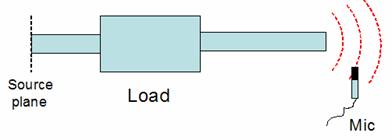
One-load method
Requires only one calibrated load and one auto-spectrum measurement as indicated in Figure 2. Fuzzy and crisp options of the method are available and are applied from a stand-alone user interface where the measured spectrum may be given discretely, or in 1/N octave bands or fixed bands in dB(L,A,B,C) units.
This method is particularly useful when the resources required for implementation of the multi-load methods described above are not available. The sound pressure level (SPL) spectrum radiated from the open end of an intake or exhaust system is customarily measured in the industry. The one-load method enables the estimation of the equivalent source characteristics from the knowledge of only such measured SPL spectrum and a block diagram model of the existing system without making blind assumptions.
Simulation of measurements
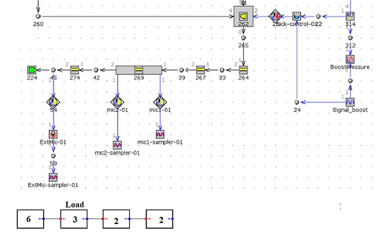
One-dimensional gas dynamics engine simulation software, the use of which is routine in the automotive industry for engine performance predictions, may be used to compute the microphone signals required by the above described source measurement methods. For example, Figure 3 shows the exhaust section of a GT-Power model of a turbocharged engine, which is setup for outputting the microphone signals required by the tests. Also shown in the figure is the block diagram model of the measurement setup, which is used for the calculation of the equivalent source characteristics in ADEM.
Acoustic parameters
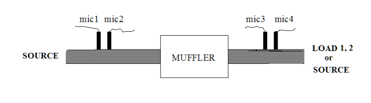
Signals recorded by the 4 microphones in the measurement setup shown in Figure 4, possibly with a mean flow, can be imported and processed in a single user interface to compute the following parameters:
Transmission Loss
The measurements are implemented in the SOURCE-LOAD 1 configuration, where LOAD 1 is anechoic.
Attenuation
The measurements are implemented in the SOURCE-LOAD 2 configuration, where LOAD 2 has the actual boundary condition.
Transfer matrix
The measurements may be implemented in either one of the following two configurations: SOURCE-LOAD 1 plus SOURCE-LOAD 2, and SOURCE-LOAD 2 plus LOAD 2-SOURCE
Reflection coefficient
The measurements are implemented in the SOURCE-LOAD 1 or 2 configuration. In this case it suffices to process the microphone signals from either pair of the microphones.
Signal analysis
A snapshot of the signal analysis interface of ADEM is shown in Figure 5. This interface may be used for signal analyses tasks such as generating various time-signal forms, importing measured time-signals, playing and recording audio signals, pre- and -post processing of discrete time-signals by the fast Fourier transform, order analysis, frequency response function calculation, signal input in sound pressure calculations, and more.

