ADEM-EDU TUTORIAL

Introduction Steps Nesting Exercises FAQs

Introduction

With adem-edu, you can study one-dimensional (plane wave) acoustics of duct systems which can be decomposed into a cascade (series) of two-port generic sub-components whose acoustic models (elements) are resident in the element database of the software.  You can obtain adequately accurate results for engineering applications involving ducts with subsonic low Mach number mean flows and of sizes less than the wavelength.  

In this tutorial, we will work with the expansion chamber shown in Fig.1.   This relatively simple duct system is chosen for the clarity of the tutorial.  No generality is lost by this, because all duct systems are modeled and analyzed by the same steps.  Incidentally, it is a real life silencer studied by Alfredson and Davies (Journal of Sound Vibration 15 (1971) 175-196).  It was mounted on the exhaust line of an i.c engine and, at the engine speed considered, the gas temperature and the Mach number of mean gas flow velocity in the tailpipe were 690 ^oC and 0.15, respectively. The atmospheric pressure is assumed to be 101000 Pa. In the actual silencer the inlet and outlet ducts and the chamber were all of circular geometry, however, since we are going to build a one-dimensional acoustic model, the actual geometry of these component are not relevant, they can be rectangular, elliptical, etc., provided that the cross-sectional areas are the same.

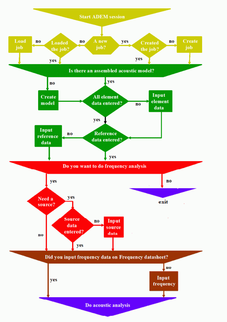
The plan of the tutorial is as follows: We will first explain the steps summarized in the above Quick Start Chart for making an acoustic model and inputting its data.  Then we will compute the Transmission Loss (TL) of the expansion chamber.  TL is the most used acoustic performance parameter, but it is often useful to look also at parameters called Attenuation, Noise Reduction, and Insertion Loss. Next, we explain how these parameters can be calculated in adem-edu. Finally, we will compute the radiated Sound Pressure Level at 0.15 m from the tailpipe outlet when the muffler is excited from its inlet pipe by a constant source.  The tutorial concludes with an example showing the activation of an additional connection node, which we call nesting node, in a two-port acoustic element, and supplementary information such as complete data summary of the expansion chamber, some exercises, and frequently asked questions.

Steps

Step 1: Create system file

Select the New option of the File menu. This opens the form shown in Fig.2, prompting you to input a name for future identification of the job file. In this case, we have called it ‘Muff1’.  All adem-edu job files are stored with the same extension ‘sf’ and are in the directory c:\adem_edu\jobdata. Once created, a job file can be opened by using the options provided in the File menu (see the online Help). The name of the current system file is displayed in the caption of the main menu window. File names are limited to 8 characters, must obey the DOS filename syntax and are case insensitive.

Step 2: Input reference data

2.1 Click on the Reference option of the Datasheets menu.  This opens the Reference datasheet form (Fig.3). Notice the Help control on the datasheet. This is a common feature of the forms you will use when communicating with computer.  By clicking on it, you can access the Help topics containing information about the use of the form and the meanings of the parameters displayed.   

2.2 Input the code number of the fluid contained in the system. The fluid conveyed in the system is defined by using a code number.  Only code numbers 1 and 9 are available in adem-edu. Fluid 1 is dry air and fluid 9 represents any fluid.  In case of dry air, no input is necessary except the code number. All relevant physical properties of dry air are computed by the program as function temperature and pressure. This capability enables the calculation of the effects of mean temperature and pressure gradients along the ducts.  In case of fluid 9, the program prompts the user to input the mean density and the speed of sound of the fluid.  The user should be aware that, this option is subject to some restrictions. Firstly, the specified density and speed of sound are assumed to be the same throughout the system. This makes the mean temperature and pressure inputs in the Reference datasheet and in all element datasheets redundant. The second limitation is concerned about the elements having sound absorbent materials or including visco-thermal effects. For such elements, it is necessary to know the fluid properties such as the shear viscosity, thermal conductivity, specific heat ratios and so on. Therefore, the use of the generic fluid option should strictly be limited to components having hard surfaces with negligible boundary layers.  The third restriction about using the generic fluid option is about liquids: the use of components with perforated pipes should be avoided, since the perforate impedance database of the program is currently limited to correlations validated for gases. 

2.3 Input the radiation node number.  In exhaust and intake systems, the open end of the system is called the radiation node (because sound is radiated from there to the exterior environment).  We must assign a positive integer as the number of this node.  Here, we have input 1 for the radiation node number. We will recall this input when numbering the nodes (connection points) of the acoustic model of the system in a later step.   In exhaust and intake systems, the open end of the system is the most convenient reference section, because the fluid and flow properties are known or can be measured accurately there.   

2.4 Input the fluid temperature and pressure and the cross-sectional area of the duct at the radiation node of the system. The mean flow velocity can be input either as Mach number, or as velocity in m/s or as mass flow rate in kg/s.  Input is required only for one of these parameters, the other two are then computed by the program.  In this example, we input the Mach number, because it is given.  Note the ‘d’ prefix in the csa input.  This prefix instructs the computer that the number following it is a diameter in mm that it is to be converted to area in m² before storing.

2.5 All essential reference parameters are now input as shown in Fig.4.  Click on the Save button. The remaining parameters on the datasheet are computed by the program. You can check the saved reference data by re-opening the Reference datasheet (see, Fig.5).

Step 3: Assemble acoustic model

It is recommended that, before proceeding with this step, the acoustic two-port elements which came with the software are reviewed.  The online Help contains detailed descriptions of the elements. The program can model any ductwork, provided that appropriate two-port building block elements are available in its element database.  

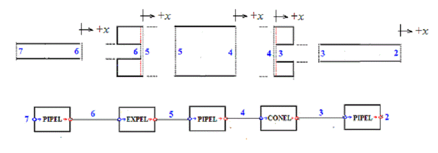
3.1 Divide the system into components.  Typical adem-edu elements are PIPEL (homogeneous uniform pipe with uniform mean flow), EXPEL (sudden area expansion) and CONEL (sudden area contraction).  The chamber in Fig.1 can be assembled from these elements as shown in Fig.6. In this figure, the components are shown schematically in an exploded view before assembly and in block diagram format after assembly.  We use the block diagram representation frequently, because it provides a clear and concise way of describing the components and their connectivity. In the block diagram, the connection sections of the components are represented by nodes.  The inlet and outlet nodes of elements are shown by small circles in blue and red, respectively (Fig.6).  All two-port elements are formulated so that the nodes represent the inlet and outlet sections of the corresponding components according to whether the positive direction of acoustic flow is into or out of the element. Thus, Fig.6 tacitly implies that the acoustic source drives the silencer from the inlet of leftmost PIPEL. This implication is independent of the direction of the mean flow direction.  So, the block diagram in Fig.6 can be an acoustic model of an expansion chamber in an exhaust line or an intake line.  The option is determined by the sign of the mean flow velocity parameter input in the Reference datasheet.  A positive input means that the mean flow is in the positive direction of the acoustic flow, signifying an exhaust flow.  If the chamber were in an intake line, the mean flow velocity parameter should have been input as a negative number in the Reference datasheet.

Note that the gaps you see in Figs. 1 and 6 (and later figures) between the dotted lines are really introduced for simplifying the visualization of the inlet, outlet, and side-branch sections. These lines are coincident in reality. So, you may assume the gap thickness to be infinitesimally thin and the element data are entered on this understanding (see Step 3.3). The same also applies when you apply end-correction. The only difference is that the extended pipe length will be different than its physical length. 

3.2 Number inlet and outlet nodes of elements. Having determined the acoustic elements from which the expansion chamber is going to be assembled from, we must next define the connectivity of these elements for the computer. This is done by giving numbers to the inlet and outlet nodes of the elements. In adem-edu, node number assignments have to be done manually by the user. Positive integers can be assigned arbitrarily as Inlet and outlet node numbers provided that: 

• connected nodes have common node numbers.
• non-connected nodes and the radiation node (see 2.2) have distinct node numbers. 

It is recommended that you keep a record of the assembly with the assigned node numbers.  A block diagram of the system (Fig.6) proves to be very convenient for this purpose.

3.3 Input element node numbers and physical data.  Element node numbers and physical data are input by using the Elements datasheet form.  You can open this form from the DataSheets/Elements menu.  It can be opened in several modes such as New, Change, Review, etc.  (see the online Help about using the features of the Element datasheet). When an element is to be initialized for the first time, it must be opened in the New mode (Fig.7). 

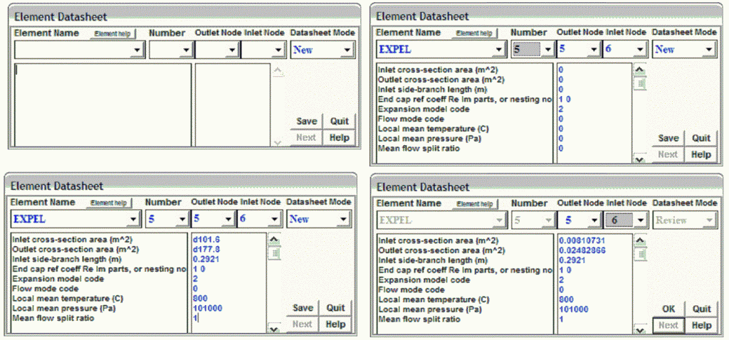
In this mode, elements can be initialized in any order desired. For example, let us initialize EXPEL in Fig.6. First, enter the inlet and outlet node numbers of EXPEL in the input windows of the drop-down lists labeled Inlet Node and Outlet Node. Then click on the drop-down list labeled Element Name and select EXPEL either by its name or number (5). This brings to view the parameters of EXPEL and their tentatively initialized values (Fig.8). To examine the definitions of the element parameters, click on the Element Help button. This opens the topic of the on-line Help containing general information and parameter definitions of EXPEL. At this point, you may Save the element with whatever data there is on the datasheet and resume the data input at a later time by opening the element datasheet in the Change mode or input some more or all of the values of the element parameters and then Save the input. Here, we have chosen to input all element data (Fig.9).  Note that, we have assumed that the local mean temperature of this element is 800 ^oC.  We will assume that the mean pressure is uniform throughout the chamber. This is plausible, because mean pressure losses are negligible and mean pressure variations do not have substantial effect on acoustic propagation. Finally, we save the data by clicking on the Save button.  The saved information can be examined by opening the Element datasheet in the Review mode and selecting inlet or outlet node number from the drop-down list of the datasheet (Fig.10). You can also edit the input by opening the Element datasheet in the Change mode.

The remaining elements in Fig.6 are initialized similarly. After all elements are initialized and the element parameters are input, it is recommended that the element data is carefully examined in the Review mode of the Element datasheet for possible typing errors, since the program contains no checks for abnormal or incorrect entries. Also note that, although you will enter the values of the length parameters as positive numbers, when element data are reviewed, you will see some of these displayed as negative numbers. These modifications are made by the program in order to comply with the sign conventions.

Step 4: Define boundaries 

The system model in Fig.6 is not complete, because the acoustic conditions at some boundaries are not defined yet. In particular, we have to define the reflection coefficient at the open end of the tailpipe, and the acoustic source driving the system.  The walls of ducts are not of concern, because they are taken care of during the mathematical formulation of elements and assumed to be solid in general, unless specified otherwise in the element description.  However, in some elements, like EXPEL and CONEL, endcaps constitute an exception.  Reflection coefficient of the endcaps of these elements occur as an input parameter in their datasheets and must be input appropriately by the user in the complex number format:

a  b  

where the first number denotes the real part of the reflection coefficient and the second number (separated from the first by one or more space) denotes its imaginary part.  In Fig. 9, this input for EXPEL is 1 0 since the endcap is assumed to be rigid (of infinite impedance). This input format is required because reflection coefficient is a complex number in general.   When an endcap reflection coefficient is input directly, it is assumed to be independent of frequency, which may not be realistic for some end-cap surfaces.  A more general method which can be used for specifying frequency dependent reflection coefficient for an endcap is nesting.  

4.1 Define the system outlet boundary. The acoustic boundary condition at the tailpipe outlet (node 2) is applied by connecting the one-port element RADEL to the open end of PIPEL representing the tailpipe, as shown in Fig.11.  With RADEL, we have also shown the radiation node number 1, which we assigned in Step 2.3.  Thus, it now transpires that the radiation node number actually represents the outlet of RADEL. However, RADEL is a one-port element; that is, it has only an inlet node for connection to other elements. The outlet node of RADEL is a conceptual node, as no element can be connected to it.  For this reason, it is not visible in the block diagram; however, you must still assign a number to it when initializing the RADEL data.

RADEL’s data are input as other elements. In fact, RADEL is a generic element for application of acoustic boundary condition (the reflection coefficient) at terminals of ductworks.  The boundary condition is specified by inputting its code number in the datasheet of RADEL. For example, 1 means an anechoic outlet, 6 means an unflanged open end with mean flow.  Also, RADEL need not always be associated with the radiation node number, but an acoustic model must always have at least one RADEL, the outlet node of which is the radiation node (see Fig.24).

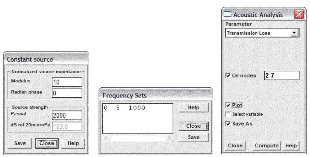
4.2 Define the acoustic source. An acoustic model of a ductwork is always associated with an acoustic source, but, as in this example, the actual source may be outside the boundaries of the system model considered.  However, we may envisage an equivalent one-port source driving the silencer from the inlet node of its inlet pipe (node 7 in Fig. 11).  This concept of equivalent source is exact, if the system is linear, which means that we can find an equivalent source acting at node 7, which produces the same acoustic field in the chamber as the actual source. In adem-edu, you can apply a Piston source or a Constant source at the equivalent source node. Characteristics of the equivalent source need not be known for the calculation of Transmission Loss, Attenuation and Noise Reduction.  For this reason, there is a third option called Undefined source, which is introduced for the convenience of by-passing source data input if we are interested in one of these parameters.  In this tutorial, we will apply a Constant source since we are going to also compute the Insertion Loss of the chamber and the Sound Pressure Level radiated from the tailpipe.  When you select the Constant source option from the DataSheets/Source menu, the program opens the form shown in Fig. 12 for inputting the normalized impedance and the pressure strength of the source.  The input on the form defines a constant source of normalized impedance 10 0 and pressure strength 2000 Pa. 

Step 5: Set analysis frequency range.

The frequency range of the analysis is input by using the Frequency datasheet, which is accessed from the DataSheets/Frequency menu. The features and use of this datasheet are described in detail in the on-line Help. Fig.13 shows the input to the Frequency datasheet for this example. This input means that, calculations will be repeated by incrementing the frequency at steps of 5 Hz up to 1000 Hz, starting at 0 Hz.  Do not press the Enter key after the last line of input (your cursor must remain at end of the last line of input).      

Step 6: Compute

6.1 Transmission Loss

• Change the boundary condition code of RADEL to 1
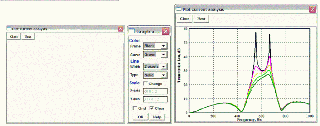
• Select the Transmission Loss option of the Analysis menu. This opens the Acoustic Analysis dialogue shown in Fig.14
• Input the system inlet node number (7) and outlet node number (2)
• If you want to plot the computed Transmission Loss spectrum, check the box labeled Plot. If you want to save the computed Transmission Loss spectrum in a text file for post-processing in Excel or similar software, check the box labeled Save As. This opens the windows system file browser to select or create the file to which the results of the calculations are to be stored as space delimited txt data. Here, the user should be aware of the following restriction: The program does not recognize directory or file names having spaces. Single names should be used to avoid error messages.
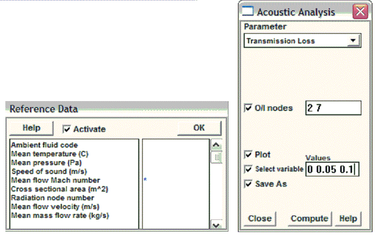
• If the Transmission Loss is required for several values of a parameter, check the box labeled Select variable. This opens a single line input window, and the Elements datasheet and the Reference datasheet are also opened for making the parameter selection. Let us compute the Transmission Loss for different values of the tailpipe Mach number, other parameters being assumed to remain the same.  Fig.15 shows the Reference datasheet with the reference mean flow Mach number activated (the parameter marked with an asterisk). Click on the OK button of the reference datasheet and input in the Select variable window the desired values of the Mach number for which the calculations are to be repeated (Fig.16).
• Click on the Compute button to start the calculations.
• If the Plot option of the Acoustic Analysis dialogue is checked, then, at the conclusion of the calculations, the program opens the Graph Attributes dialogue (Fig.18) and the ‘Plot current results’ form (Fig.17).  Graph Attributes dialogue contains controls for selecting the vertical and horizontal axes scales, line color, width, and type. If you click on the OK button, the computed spectrum is plotted using the default settings of the controls. If calculations are carried out for several values of a selected parameter, the first plot corresponds to the first value of that parameter. To plot the spectrum computed for the next value of the selected parameter, click on the button labeled Next. This will re-open the Graph Attributes dialogue to repeat the plotting process (Fig.19).  Please refer to the online Help for detailed description of the use of the Graph Attributes dialogue.

6.2 Attenuation

The procedure is the same as Transmission Loss, except that the boundary condition code of RADEL may now be changed to 6 since Attenuation is usually computed by using the actual boundary condition at the open end. 

6.3 Noise Reduction

Noise Reduction can be calculated as NR, NRSWM and NRO (see the online Help).  These are computed as Attenuation, but with following differences: 

NR: The inlet and outlet nodes need not be the source plane and tailpipe outlet nodes. 

NRO: Additional input is required to define the microphone location. These are input on the Acoustic Analysis dialogue.

NRSWX: The inlet and outlet nodes must be the inlet node (node 7) of the inlet pipe and the outlet node must be the inlet node (node 3) of the tailpipe.

6.4 Insertion Loss

• Change the boundary condition code of RADEL to 6
• Select Constant source and input the normalized source impedance (Fig.12). You will also be required to input the source pressure strength, but this need not be precise, because it is not used in calculations.
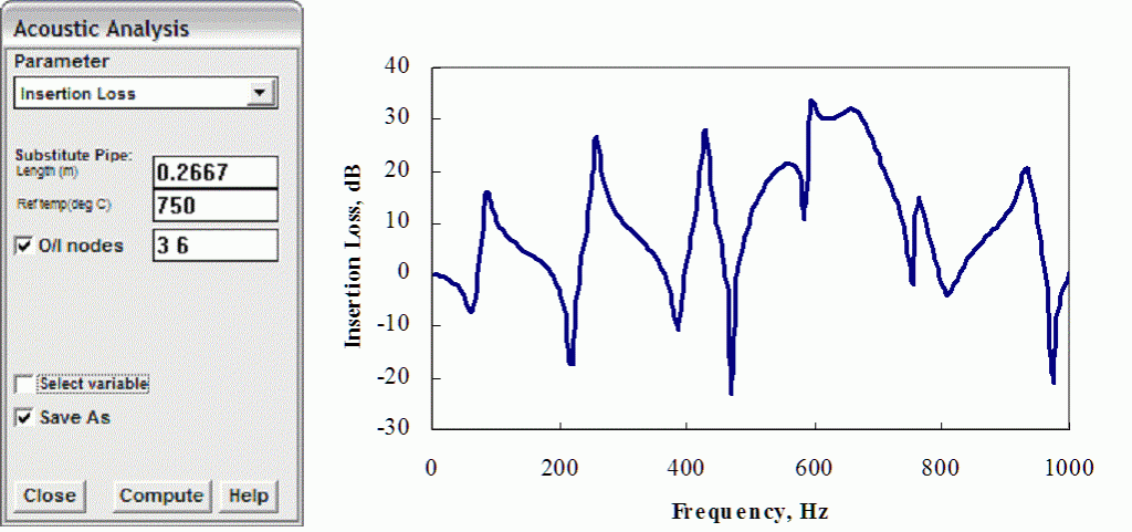
• Input the length of the substitute pipe and its mean temperature (Fig.20).  Insertion Loss is computed by replacing the chamber by a straight pipe of the same diameter as the tailpipe.  In this example the substitute is taken as a uniform pipe that joins the inlet and outlet extensions.  This is made possible by the fact that nodes 6 and 3 are available in the acoustic model.  A longer substitute pipe could be used if the acoustic model had nodes for its connection.  Such nodes may be introduced by modeling the inlet and outlet pipes as cascade of two or more pipe elements, but this is really not warranted for homogenous pipes.
• Input the inlet and outlet nodes of the chamber proper (see, Fig.20). The source plane and the tailpipe outlet nodes are determined by the program.
• Click on Save As and/or Plot checkbox.
• Click on the Compute button and save or plot the results as described for Transmission Loss. Fig.21 shows the computed Insertion Loss (M=0.15) as plotted in Excel.

6.5 Sound Pressure Level

• Change the boundary condition code of RADEL to 6
• Select Constant source and input the source parameters.
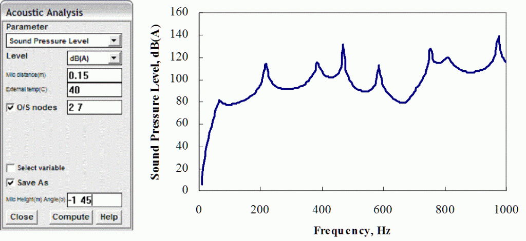
• Open the Acoustic Analysis dialogue (Fig.22)
• Select the level filter
• Input microphone distance, height, and angle. Microphone height is relevant if the tailpipe is radiating to a hemi-anechoic field. In this example, the radiation is assumed to be into a free field. This is invoked by inputting any negative number for microphone height.
• Input the environment temperature in the vicinity of the microphone.
• Input the source plane and tailpipe outlet node numbers (7 and 2)
• Select SaveAs and/or Plot and click on the Compute button. The computed Sound Pressure Level is shown in Fig.23.

Nesting 

Some two-port elements like EXPEL may have a connection node other than their inlet and outlet nodes. Such a node is called nesting node.  

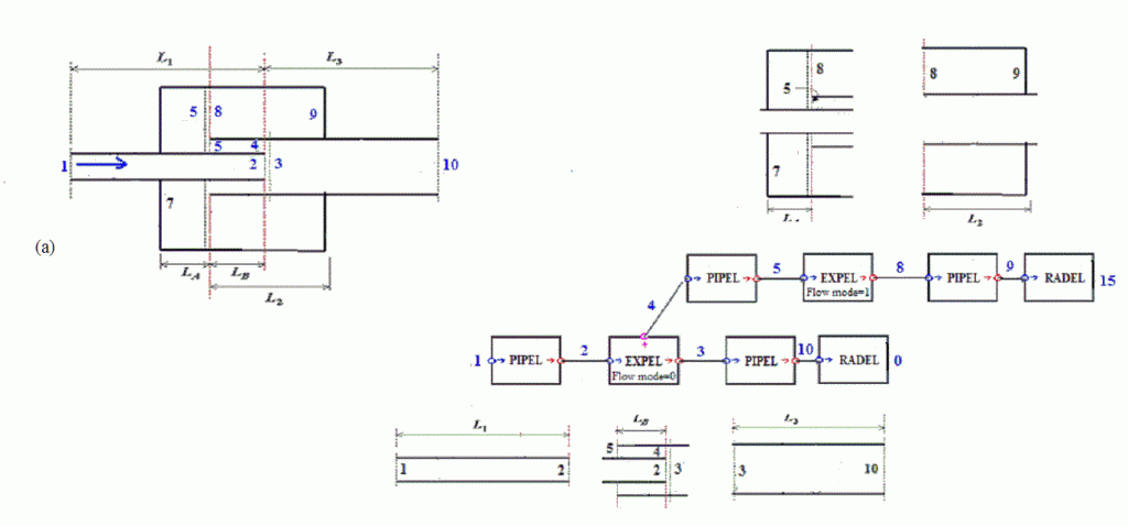
Consider the folded resonator with rigid endcaps shown in Fig. 24a.  This resonator can be exploded into the components which are shown at the right of the figure in line with the elements of the assembled block diagram of the resonator.  Elements with inlet/outlet nodes 1/2, 3/10, 4/5 and 8/9 are pipes and are modeled by PIPEL. Component 5/8 is a flow reversing expansion and is modeled with EXPEL. So, the problem is the modeling of the acoustic wave transfer from node 2 to node 3. If the reflection coefficient of node 5 were known, this could have been done by using EXPEL. But the reflection coefficient at node 5 is not known. However, EXPEL may still be used because it has a nesting node. This means that the branch of EXPEL can be referred through an arbitrary cascade of two-port elements to a boundary of known reflection coefficient. In this case, the cascade path is 4-5-8-9 and node 9 has known reflection coefficient, since it is a rigid end-cap.  This feature (called nesting) of EXPEL (and other two-port elements) can be activated simply by inputting for the element parameter ‘reflection coefficient’ on its datasheet, the inlet and outlet nodes of the branch cascade path separated by a space(s). In this case, the input is 4   9, which are the inlet and outlet nodes, respectively, of the cascade 4-5-8-9.  But you must select both these node numbers greater than 3 in order that the program does not take them for a reflection coefficient input.   

The block diagram of the resonator is shown in Fig.24. The elements of this model are initialized as described in the previous parts of the tutorial and acoustic calculations are carried out also similarly. It should be noted that, this system model contains two RADEL elements. The RADEL in the nesting cascade has boundary condition code 5 and models the rigid endcap at node 9.  Its hidden outlet node number is 15, but this is not a radiating node, since it is closed. The RADEL on the main cascade models the open end of the resonator.  Its hidden outlet node number, 0 (zero), is the radiating node of the resonator.  

Exercises

1. The element database contains an element called TFCHAMBER.  You can model the expansion chamber in Fig.1 without exploding it into sub-components by using this element.  Make an acoustic model of the expansion chamber in Fig. 1 by using TFCHAMBER, run it with the same data and compare the results you get for TL, IL and SPL  with the corresponding spectra shown in the tutorial.

2. The element database contains an element called FOLDEXPEL.  This element models the folded resonator shown in Fig. 24a.  You will find an acoustic model of this resonator constructed by using FOLDEXPEL loaded in the job directory of adem-edu with name FOLDEXP.  Open this file from the File/Open menu. Examine the input data and run it to compute the Transmission Loss of the resonator. Warning: The node numbering in the FOLDEXP file may be different than the numbering shown in Fig. 24. In adem-edu, avoid using 0 (zero) as a node number.

3. Make an acoustic model of the folded resonator in Fig. 24a by using the exploded elements shown in Fig.24.  Assign node numbers to the elements and determine the values of the parameters of the elements from the input data of the acoustic model in Exercise 2.  Input this data in your acoustic model and run the model to compute the Transmission Loss of the resonator. Compare your results with the spectrum obtained in Exercise 2.

4. Repeat Exercises 2 and 3 for Insertion Loss and Sound Pressure Level. 

5. You can compute several acoustic performance parameters with adem-edu.  Normally, Insertion Loss is the most useful parameter when designing a silencer, but its computation will be problematic because of lack of information about the source pressure strength and impedance (or the source impedance if the substitute pipe method is used). Then a possible three-step procedure to follow is: 

1. Compute Transmission Loss and make sure that your design is ok at the critical frequencies (usually the major engine orders).

2. Compute Attenuation and observe that noise reduction at the critical frequencies are not affected by tailpipe reflections appreciably.

3. Compute Insertion Loss by assuming different values for the normalized source impedance.  The variations should give an idea about the likely values of Insertion Loss.  A typical value used for normalized source impedance for car exhaust silencers is (1+i)/sqrt(2), where i denotes the unit imaginary number.  Source impedance is in general frequency dependent, but Insertion Loss is not overly sensitive to it.  

Evaluate the efficacy of the above-described procedure for the expansion chamber example considered in this tutorial.

Expansion chamber data

Element name               EXPEL          
Element number                                        5
Outlet and inlet nodes                             5 6
Inlet cross-section area (m^2)        0.0081073
Outlet cross-section area (m^2)   0.02482866
Inlet side-branch length )               0.2921
End cap ref coeff Re Im parts, or nesting nodes 1 0
Expansion model code                                   2
Flow mode code                                          0
Local mean temperature (C)                           800
Local mean pressure (Pa)                              101000
Mean flow split ratio                                   1

Element name               RADEL          
Element number                                          6
Outlet and inlet nodes                                  1 2
Radiation cross-section area (m^2)                      0.00810731
Boundary condition code                                 6
Radiation temperature (C)                               690
Local mean pressure (Pa)                                101000
Mean flow split ratio                                   1
External environment temperature (C)                40

Element name               PIPEL          
Element number                                          2
Outlet and inlet nodes                                  2 3
Pipe cross-section area (m^2)                           0.00810731
Pipe length (m)                                         ¯0.6985
Local mean temperature (C)                              690
Local mean pressure (Pa)                                101000
Mean flow split ratio                                   1
Slip flow parameter                                     1

Element name               CONEL          
Element number                                          4
Outlet and inlet nodes                                  3 4
Inlet cross-section area (m^2)                          0.02482866
Outlet cross-section area (m^2)                         0.00810731
Outlet side-branch length (m)                           0.2286
End cap ref coeff Re Im parts, or nesting nodes         1 0
Contraction model code                                  4
Flow mode code                                          0
Local mean temperature (C)                              690
Local mean pressure (Pa)                                101000
Mean flow split ratio                                   1

Element name               PIPEL          
Element number                                          2
Outlet and inlet nodes                                  4 5
Pipe cross-section area (m^2)                           0.02482866
Pipe length (m)                                         ¯0.2667
Local mean temperature (C)                              750
Local mean pressure (Pa)                                101000
Mean flow split ratio                                   1
Slip flow parameter                                     1

Element name               PIPEL          
Element number                                          2
Outlet and inlet nodes                                  6 7
Pipe cross-section area (m^2)                           0.00810731
Pipe length (m)                                         ¯0.7921
Local mean temperature (C)                              800
Local mean pressure (Pa)                                101000
Mean flow split ratio                                   1
Slip flow parameter                                     1

Frequently asked questions

I’m using only the Transmission Loss (TL) because I don’t have any information about the source impedance. I saw some methods to measure the source impedance, but none of them seemed feasible with the kind of equipment we have available. Do you think that carrying on the design using Transmission loss is a major issue?

Answer: This is particularly critical when designing large industrial silencers, because you will not normally have a chance for making prototypes and what you design must work the first time.  So how should a practicing engineer should proceed?  See Exercise 5 for a 3-step procedure. If the sound pressure level radiated from the tailpipe, or snorkel, is given, the source characteristics can be estimated without wild guesses by using the one-load method.

When I was using the software to compute the insertion loss, I had some doubts about the parameter substitute pipe length. In the Tutorial, was the length used between the input and output extensions, for any specific reason? Could you explain more about what exactly the software is doing with this parameter.

Answer: When you use the substitute pipe method, the program assumes that the equivalent source pressure strength and impedance are not altered.  Then insertion loss becomes independent of the source pressure strength and you need to input only the source impedance (see on-line help on Insertion Loss). As long as you have a uniform lossless pipe between the equivalent source plane (the pipe section from which you imagine the silencer is excited) and the tailpipe outlet plane, it is not important how you select your substitute pipe, provided that your acoustic model contains nodes to insert this pipe in between, as in the Tutorial example. Then you do not have to worry about the location of the equivalent source plane.  If the inlet and outlet ducts are not in line or have different diameters, the definition of substitute pipe is not so precise, but the basic idea is the same, that is, to connect the equivalent source plane by a lossless uniform substitute pipe to the tailpipe.  To do this, it may be necessary to introduce an area change or use a slightly curved duct and assume that effects of these may be neglected for practical purposes.

Why the lengths of the inlet and outlet pipes used (in the tutorial) are not the same as the ones in the figure 1. For example: The inlet pipe is 0.5 m in length, and it was used 0.7921 m. This appears to be the sum of the pipe and the inlet extension lengths, but the length of the extension is already inside the EXPEL element.

Answer: The figure serves to show the dimensions of the muffler, not the lengths of the pipes in the acoustic model.  Lengths in the acoustic model are determined by the nodes you want make accessible.

While I was studying element 8, I saw that the software allows me to choose between different theories for the hole impedance in Grazing Flow. I tested the different models and saw that they give different results. I was wondering if you could suggest one that is good for using with large porosity (more than 10%).

Answer: Software gives you the alternatives people have proposed previously.  As you can see from the variety of them, there is not one solution.  You will have to exercise your own judgement to pick the one best suited to your application. However, here are some general guidelines: A model which gives unstable results in desired frequency ranges should be avoided. Any of models which yield consistent results for frequencies of interest may be used.  When porosity is larger than 10%, a perforated section will be transparent to low frequency sound waves.  This means that you should be getting results similar to that of the expansion chamber which you obtain when you cut out the perforated section.  You can use this feature to test the efficacy of a model for relatively large porosities. In my experience, model 3 generally gives good results when there non-negligible grazing mean flow. It reduces to the classical model 1 when there is no mean flow. Finally, note that it is the hole diameter and mean flow, not porosity, which determine the efficacy of a model.

When I was computing Insertion Loss (IL) I realized, by making some tests, that the length of the pipe before the chamber has a certain influence on the IL results. But my question is, in practice what I have before the chamber is a complex system of ducts and devices, far from being a straight pipe, how usually this is taken into consideration? For example, in a turbocharged Diesel engine I would have the turbine and the intake manifold before the chamber.

Answer: The length of the pipe before the chamber is important, because its inlet determines your equivalent source plane and your calculations assume that the characteristics you use for the source are the equivalent source characteristics at that plane.  If you take the equivalent source plane elsewhere, for example at the outlet of the turbine, then you will have to include all components downstream of it in your acoustic model and use the equivalent source characteristics at the outlet of the turbine. The model will now be too complex to apply the substitute pipe method.  Therefore, you will have to compute IL loss of the chamber by doing two SPL calculations, one with the acoustic model of the system not including the chamber proper and one with acoustic model including it and subtracting the computed SPL spectra. So, taking the ESP at the inlet of the chamber simplifies the calculations substantially.  In practice, it is much simpler to measure the source characteristics at the inlet of the silencer than at a place like outlet of the turbine.  So, if you can make measurements, then you need not be concerned about the components upstream of the chamber.  In the absence of this capability, all you can do is to make guesses about the source impedance and observe the sensitivity of the results as you vary the source impedance and hope that the actual value (which is frequency dependent) is included in these variations.

I was thinking about a silencer like the element 8 but using a rectangular perforated duct instead of a circular one. Would it be better or worse than the circular duct?

Answer: You can still model a through-flow silencer with rectangular perforated pipe in adem_edu by using element 8.  You see, in 1-D, the shape of the actual pipe sections is not important; non-circular ducts can be modeled as circular ducts of the same csa and porosity, if perforated. You can use element 19 similarly, if annulus is packed.